AlphaZero Connect-4 Bot

Overview

I implemented AlphaZero, a reinforcement learning algorithm designed by Google DeepMind, and trained it to play Connect-4. It uses a neural network combined with Monte Carlo Tree Search to both learn the game and play it. The original paper trained AlphaZero to superhuman levels of Go and Chess, but this is not feasible without large amounts of hardware. Instead, I was able to achieve a decent bot for Connect-4 that is on-par with my own skill level after around one day of training.

The algorithm is built around a neural network that takes the board state as input and outputs a policy and a value. The policy is a probability distribution over possible actions, where stronger actions have higher probabilities associated with them. The value is an estimate of who will win the game starting from the given state (\(+1\) for win, \(0\) for about even, \(-1\) for loss). These outputs are used to help guide a Monte Carlo Tree Search (MCTS) that determines the next move given a board state.

The network is trained over many stages, where each stage consists of a self-play session, a training session, and finally an evaluation session. In the self-play session, the network plays against itself many times and records data associated with each state it encountered in the games. In the training session, we use the collected data to hopefully improve the neural network weights. Finally, in the evaluation session, we play many games between the new network and the best-so-far, and update the best-so-far if the winrate is higher than a certain threshold.

My implementation can be found at this Github repository.

Neural Network

The neural network takes in a board state \(x\) and outputs a policy \(\vec{\pi}\), which is a 1d probability vector, and a value \(v\), which is a scalar:

\[f(x)=(\vec{\pi}, v).\]

\(x\) is the current placements of the pieces on the board. It’s encoded as two \(6\times7\) arrays stacked on top of each other, where each of the \(2\) layers represents the positions one of the players’ pieces: \(1\) if they have a piece there and \(-1\) otherwise.

For the network \(f\), I used a convolutional neural network. It starts with several residual blocks and splits into two output heads made of fully connected layers. The two heads are the policy head, which generates a length \(7\) probability vector over possible moves (columns on the Connect-4 board), and a value head, that generates a scalar representing the expected winner of the game. This scalar ranges from \(-1\) to \(1\), where higher values mean the current player has a stronger position and is thus more likely to win.

Move Selection with MCTS

In an actual game, we use a Monte Carlo Tree Search guided by the neural network to pick moves. It works as follows: we start with an empty search tree containing just the root node, which represents the current state. Each edge in the tree represents taking an action \(a\) starting from some state \(s\). Each edge also stores three values:

\(Q(s,a)\) is the expected outcome of the game after going along this edge, from the perspective of the player who has to move in state \(s\). This is maintained to be the average of all the values we ended up with after traversing this edge.
\(N(s,a)\) is the number of times we have traversed this edge so far during the search.
\(P(s,a)\) is the probability from the policy outputted by the neural network for state \(s\). This is calculated once and never modified. When we make a new node, the \(Q\)’s and \(N\)’s are initialized to 0, and the \(P\)’s are assigned values based on the neural network output.

Our search tree currently only contains one node, but now we start to expand it. To do this, we repeatedly traverse the tree from the root down a chain of children until we hit a node that we haven’t seen before. We then add this new node to the search tree, and repeat the process from the root again.

Each time we traverse the tree, we increment the \(N(s,a)\)’s for the edges along the path we traverse. In addition, we use the neural network to evaluate the state at the new node we add. The value returned by the neural network is propagated upwards, such that the \(Q\)-values of the edges we passed through are maintained as the average value we ended up with each time we traversed that edge.

The rule for picking children is to pick the one that maximizes the following score:

\[score(s,a)=Q(s,a)+c_{puct}P(s,a)\frac{\sqrt{1+\sum_b N(s,b)}}{1+N(s,a)},\]

where \(c_{puct}\) is a constant (for my bot I picked \(c_{puct}=1\)). This constant controls how much exploration the MCTS does. The higher it is, the more likely we are to try actions that don’t already have high \(Q\)-values.

Here are the reasonings behind the \(score\) formula:

Actions resulting in higher \(Q\)-values are favored, meaning we’re more likely to explore actions that have better expected outcomes.
We favor actions that have high policy probabilities, as the neural network is likely to assign higher probabilities to stronger actions.
The fraction in the second term favors moves that we haven’t explored as much.
As a state \(s\) gets explored more and more times, the numerator of the fraction grows slower than the denominator because of the square root. This means the second term will become less and less significant, leaving the score dominated by the first term. This reflects the increased confidence we have in the accuracy of the \(Q\) value.

Note: there is a difference between the formula I used and the one used by the original paper, which is that I added \(1\) to the summation under the square root, whereas the proposed formula doesn’t have this addition. My reasoning for this is to correct the behavior for the case where \(s\) doesn’t have any children yet. In this case, the \(\sum_b N(s,b)\) part would be \(0\), and \(Q(s,a)\) would be \(0\) as well, making the entire score \(0\) for every leaf node. This would mean exploration would be completely random for the first step, which didn’t make sense to me.

After traversing the tree a bunch of times, the visit counts for the root node are a good indicator of how good the actions are. Actions with more visits are probably stronger. Thus, by dividing each visit count by the total number of visit over all actions, we get an “improved policy” which is probably better than the original policy obtained from passing the root state into the neural network. As we’ll see later, this improved policy will be used to train the neural network to converge towards better policies. I was initially confused about why we’re using the \(N\)’s rather than the final \(Q\)-values to get the improved policy, but I realized this makes more sense since \(Q\)-values can be negative, so it doesn’t make logical sense to try to form probability distributions out of them.

The final pseudocode for MCTS looks like this:

def traverseTree(state):
    if isGameOver(state):
        return -getOutcome(state)
    
    if state in visited:
        action = getHighestScore(state) # Using the scoring function from before
        value = traverseTree(getNextState(state, action))
        
        w = N[state, action] / (N[state, action] + 1)
        Q[state, action] = Q[state, action]*w + value*(1-w)
        N[state, action] += 1
        
        return -value
    else:
        visited.add(state)

        policy, value = nn(state)
        Q[state] = [0, 0, ..., 0]
        N[state] = [0, 0, ..., 0]
        P[state] = policy

        return -value

def MCTS(state):
    for i in range(num_traversals): # num_traversals is a constant
        traverseTree(state)
    
    improved_policy = normalize(N[state])
    return improved_policy

One more thing to observe is that we’re always negating the return value. This is because traverseTree is supposed to return a value from the perspective of the other player, not the one who is currently supposed to move. For example, if the state is a losing state, we should be returning a positive value, and if the state is a winning state, we should be returning a negative value. In accordance with this, return value of getOutcome is \(1\) for a win, \(0\) for a draw, and \(-1\) for a loss, all from the perspective of the current player.

Training

We train the network by providing input/output pairs to learn from. In other words, we need to provide it with

\[(\text{game state}, \text{policy}, \text{value})\]

samples, and then use standard backpropagation to update the network weights.

These tuples can be obtained via self-play. For each game the bot plays against itself, we record each intermediate game state and improved policy it computed, as well as the final outcome:

def selfPlay():
    game_history = []
    state = State()

    while True:
        if isGameOver(state):
            outcome = -getOutcome(state)
            break

        improved_policy = MCTS(state)
        game_history.append([state, improved_policy, None])

        improved_policy = 0.75*improved_policy + 0.25*dirichletNoise()
        action = randomSample(improved_policy)
        state = getNextState(state, action)
    
    # Fill in the value part of each element in game_history
    for i in reversed(range(len(game_history))):
        game_history[i][2] = outcome
        outcome *= -1

We added some random noise to each improved policy. The main purpose of this is to encourage exploration, so that we have more diverse data to train with. The original paper uses Dirichlet noise with a parameter of \(0.03\), which I copied.

Also, the value field of each tuple is alternating. This reflects the idea that the players are taking turns and have opposite evaluations for the outcome of the game.

Each call to selfPlay generates a list of tuples the neural network can train from. We call selfPlay many times, in my case \(100\), and combine all the lists into one giant list to train with. I used a batch size of \(32\) and trained for \(30\) epochs.

After training, we check to make sure the network has actually improved. We do this by pitting a bunch of games between it and the best network we have created thus far. If it wins more than \(51\%\) of them, we update the best network. This ensures that we don’t accidentally make backwards progress. When running these games, we pick the argmax of the policies rather than randomly sampling them. We also add a small amount of Dirichlet noise so that there is still non-determinism. I wasn’t able to figure out what the original paper did to introduce randomness, so this was just a makeshift solution.

Finally, we repeat everything described above many times and wait for the network to improve. The final training loop looks like this:

nn = NeuralNetwork()
optimizer = optim.Adam()
best_nn = copy(nn)
best_optimizer = copy(optimizer)

while True:
    samples = []
    for i in range(100):
        samples += selfPlay()
    
    train(nn, optimizer, samples)

    if calcWinrate(nn, best_nn) >= 0.51:
        best_nn = copy(nn)
        best_optimizer = copy(optimizer)
    else:
        nn = copy(best_nn)
        optimizer = copy(best_optimizer)

Results

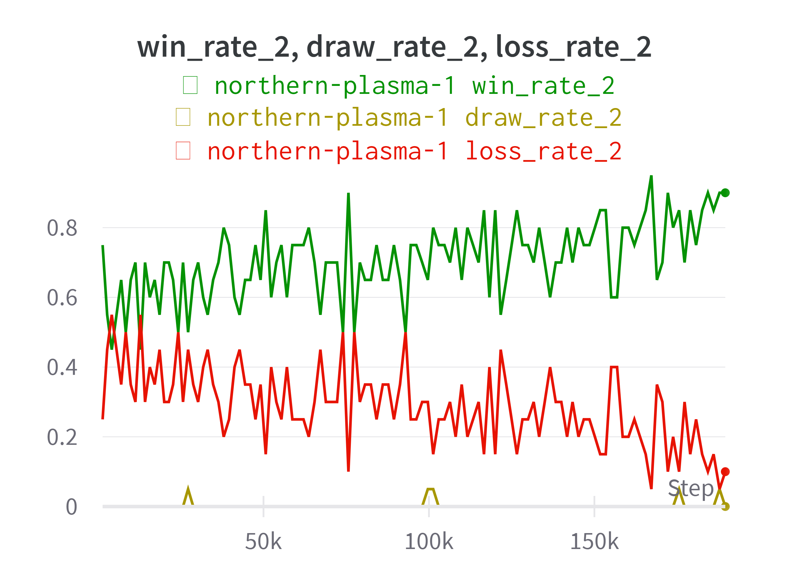
One way to measure the improvement of the neural network is to keep pitting it against the first version before any training and see if the winrate keeps increasing. The original authors had a more sophisticated elo system to evaluate the strength of the bot, but that would be overkill for this project. Here is a graph of win rate, draw rate, and loss rate of the network against the first version, over many training loop iterations. Note that I messed around a lot with different parameters and architectures, each with different degrees of success.

Winrate vs before training

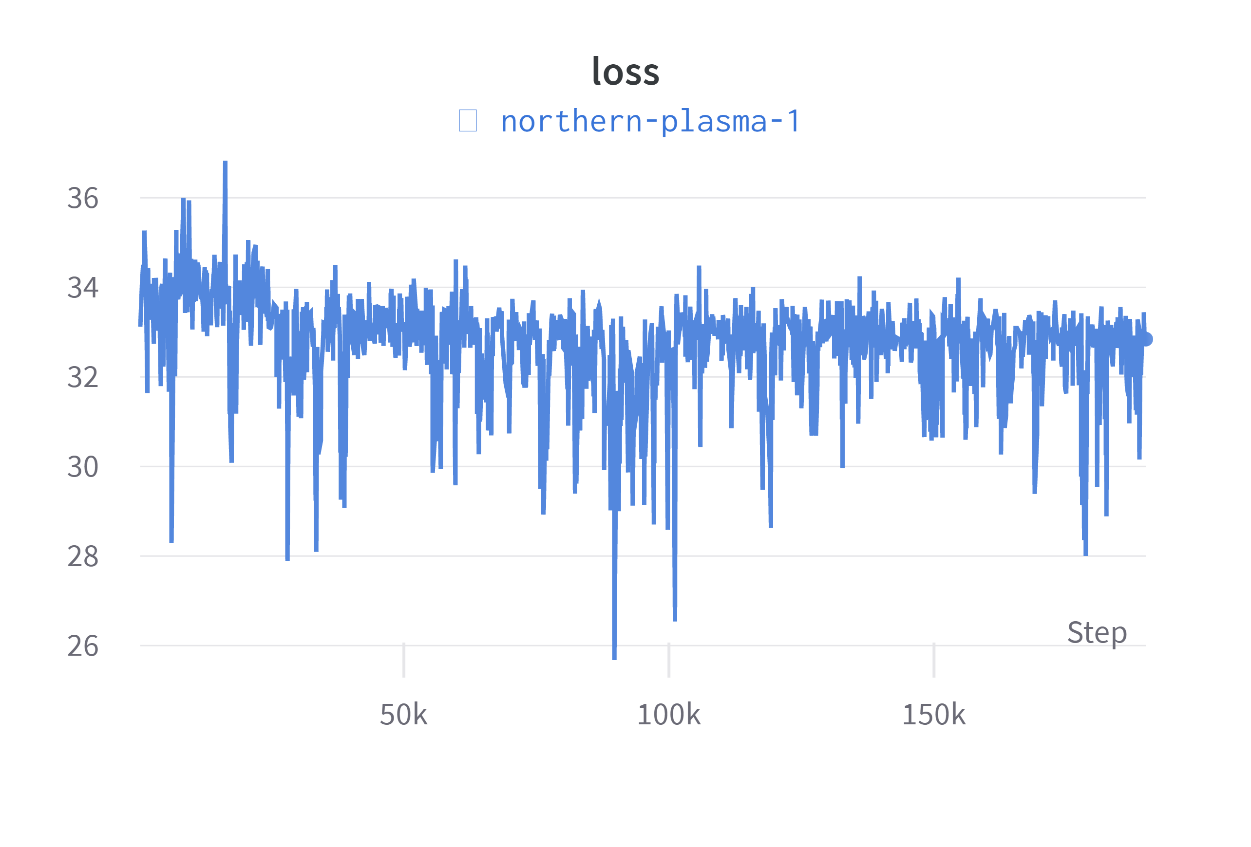
We can also observe the loss decreasing over time. Loss

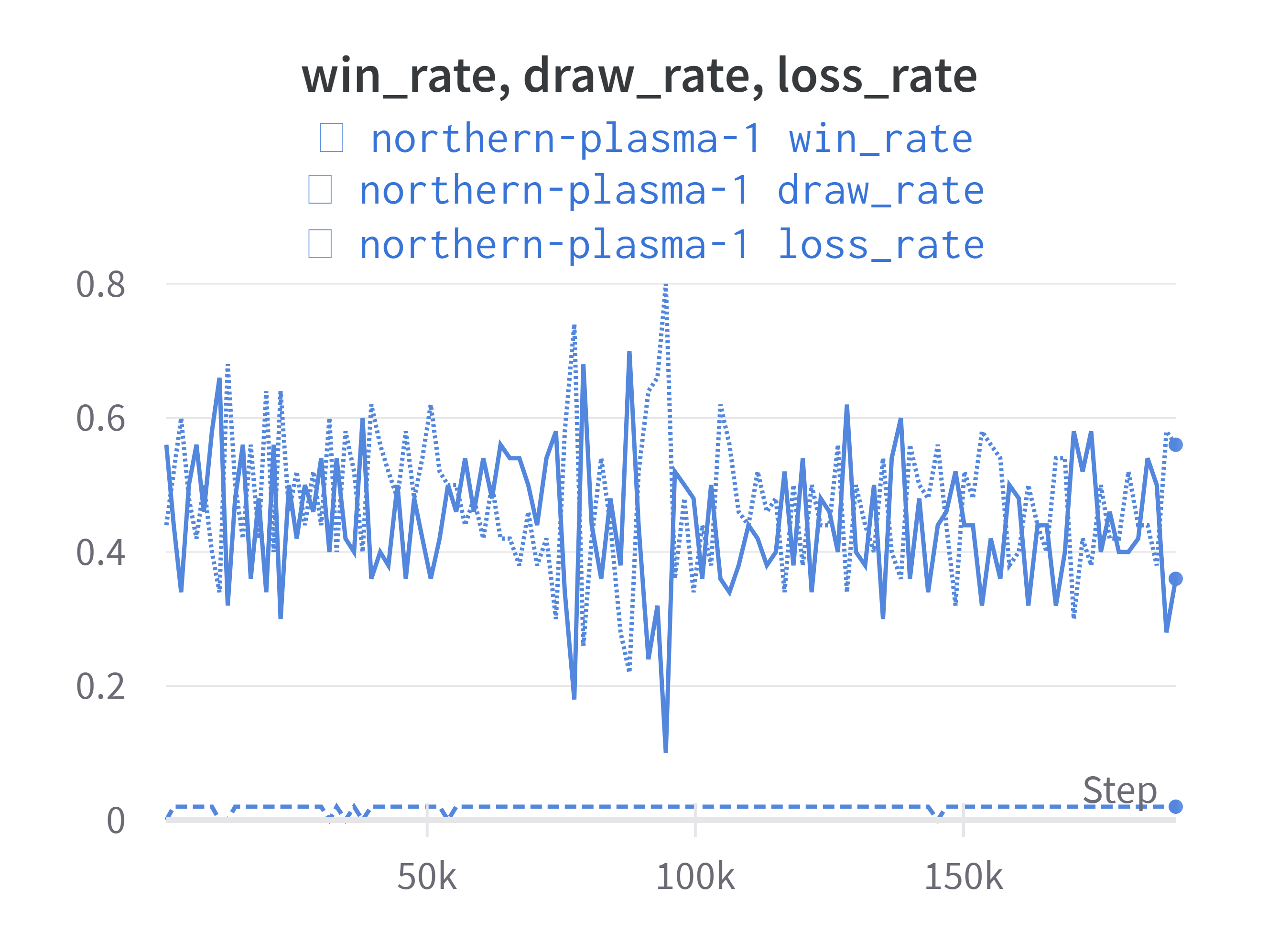
Finally, we expect that the winrate against the best-so-far should stay near \(50\%\), and never have a long decreasing trend. Winrate vs best-so-far

Credits

I used the original AlphaZero paper, this excellent tutorial and Howard Halim’s implementation as references.