Project Proposal
Konwoo Kim & Lawrence Chen
Summary
We are planning on implementing real-time position-based fluids following the 2013 SIGGRAPH work by Matthias Müller and Miles Macklin. Position-based fluids combine ideas from SPH (smoothed particle hydrodynamics) and position-based dynamics to provide stable, real-time results for incompressible fluids. We will benchmark our results on GPU with CUDA kernels vs. CPU, and present a live demo of fluid simulation at the poster session.
Background
We’re interested in the problem of efficient simulation of incompressible fluids e.g. fluids with constant density. Existing approaches to this problem like SPH (smoothed particle hydrodynamics) correctly enforce incompressibility but are sensitive to density changes and require small time steps. Instead, position-based fluids attempt to solve the problem using a PBD (position based dynamics) framework which is more stable and allows for larger time steps as well as real-time applications.
The basic idea is that given an arbitrary particle and its neighbors, we iteratively enforce the constraint that the particle density at its position stays near a constant, resting density (the definition of an incompressible fluid). A SPH density estimator applies a smoothing kernel over the neighboring particles to estimate the effect on the fluid density of the original particle. Then, we iteratively compute how we should change the positions of each particle such that the effect on the fluid densities leads to the constraints being satisfied. Concretely, the PBD framework does this by projecting particles and taking Newton steps along the constraint gradient until convergence.
The simulation loop of the full algorithms is shown below.
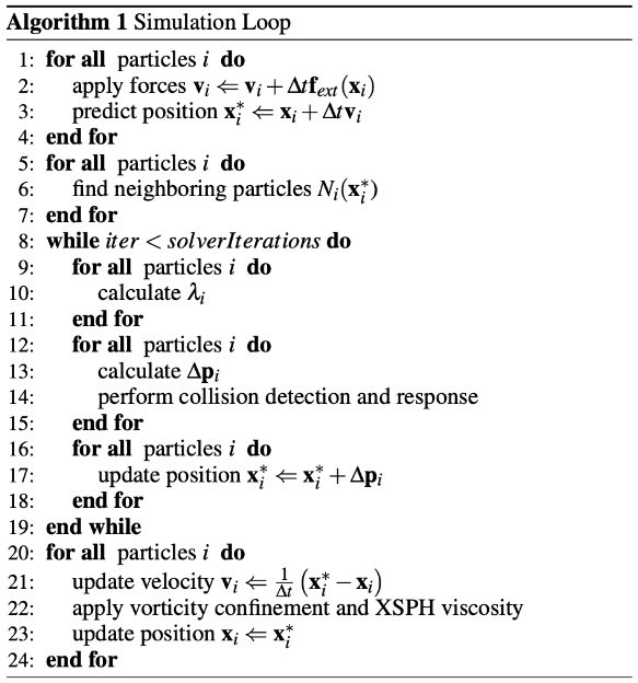
There are several key areas of the algorithm which can benefit from parallelism. These include finding neighboring particles, particle position updates, and Jacobi updates of the constraints. A naive computation of finding neighboring particles will take O(n^2) time for n particles and make real-time simulation infeasible. This can benefit from parallelism if we leverage a space-dividing data structure to efficiently compute the neighbors, although this data structure must be dynamic and handle particle movement over time. The particle position updates can also benefit from parallelism as we can parallelize the computation of the SPH density estimator over neighboring particles as the kernel is thresholded and over the grids in our data structure. Finally, the gradient computations for the Jacobi updates of the constraints can be parallelized across distinct constraints.
The Challenge
We plan to exploit parallelism for two parts of our algorithm.
Part 1: Dividing the 3d space into a uniform grid and assigning particles to each cell.
At the beginning of each time stamp, we need to create a data structure that lets us quickly query for other particles in the surrounding area. Based on previous work, we decided to assign particles to a uniform grid where each cell has size h x h x h. Then, in order to get a list of all particles that are within h of our current particle, we can quickly rule out all particles that are not in the current particle’s cell nor the 26 surrounding ones.
The main challenge for this part comes from the way our data structure is represented in memory. We could use a 3D array of vectors where each vector contains the particles for a particular cell. However, this has poor spatial locality because there is a lot of empty space in the middle of the data.
Instead, we will be storing this grid as two 1D arrays: P, the sorted particle positions, and L, the integer offsets. Elements P[0..L[0]-1] correspond to the particles in cell (0,0,0), P[L[0]..L[1]-1] correspond to cell (0,0,1), etc.
As a consequence of this special format, implementation will be less straightforward. To generate P, we plan to first create a list of positions, then sort it based on the cell indices. The sorting algorithm will be a parallel counting sort with three stages:
- Generate an 1D array counts containing the number of particles in each cell.
- Compute the prefix sum of counts; this will be L.
- Use L to place each particle in the correct slot of P.
After this part finishes, we now have an easy way to query for nearby particles, and can continue to the next part.
Part 2: Updating the position of each particle based on its environment.
Next, we need to calculate the new position of each particle after the timestep. There are multiple steps to this as described in the Background section.
This would be relatively straightforward to implement in OpenMP, but the main challenge is that we chose to use CUDA since CUDA threads have less overhead and we can spawn more of them. More specifically, the difficulty comes from the fact that particle updates depend on nearby particles. Due to its size, the full list of particle positions needs to be stored in global memory, and it would be really slow to do computation directly from that. Thus, we need to exploit shared memory in some way.
To solve this problem, we came up with the idea of assigning thread blocks to cells in the 3D grid. Each kernel launch corresponds to a single cell, and each thread within the kernel is responsible for a single particle. The benefit of this approach is that all the particles in a given cell can be updated based on just the particles in the 27 surrounding cells. This list will be small enough to be stored in shared memory rather than keeping it in global memory.
Resources
- Types of Computers
- We will have access to CPUs and GPUs on the Gates clusters and PSC.
- Gates cluster
- CPU: Intel® Core™ i7-9700 Processor @3.00-4.70 GHz
- GPU: NVIDIA GeForce RTX 2080 B (8 GB of GPU memory)
- PSC
- CPU: AMD EPYC 7742 64-Core Processor @2.25-3.40 GHz
- GPU: NVIDIA V100 (16-32 GB of GPU memory)
- We are starting our code base from scratch, but we will reference the following papers throughout our implementation. We will focus on building our implementation following the algorithm described in the first paper and implement the others in our stretch goals.
- Macklin, Miles, and Matthias Müller. "Position based fluids." ACM Transactions on Graphics (TOG) 32.4 (2013): 1-12.
- R. Hoetzlein, 2014. "Fast Fixed-Radius Nearest Neighbors: Interactive Million-Particle Fluids", GPU Technology Conference (GTC), Santa Clara, CA.
- Goswami, Prashant, et al. "Interactive SPH simulation and rendering on the GPU." (2010): 55-64.
- We will also use OpenGL tutorials for the initial rendering of the particles.
Goals and Deliverables
Our baseline goals are to implement:
- Position-based density constraints and collision constraints
- Parallelized Jacobi iteration for updating particle positions (with CUDA kernels)
- Efficient neighbor computation using parallel counting sort (with CUDA kernels)
- Parallelization of particle and constraint updates (with CUDA kernels)
- XSPH viscosity post-processing for coherent motion
- 3D Particle rendering using OpenGL
- Benchmarking of parallel vs. sequential versions on GPU vs. CPU
We plan on presenting a real-time demo of our fluid simulation at the poster session.
Our stretch goals are to implement:
- Surface tension correction to reduce particle clustering
- Vorticity confinement to reduce numerical damping
- Extend the neighbor computation to use parallel radix sort (with CUDA) following the work of Fast Fixed-Radius Nearest Neighbors
- Realistic rendering by implementing the GPU voxel rendering pipeline from Interactive SPH Simulation and Rendering on the GPU with CUDA kernels and GLSL shaders
Platform Choice
We will be using C++ for the implementation of the sequential simulator, CUDA kernels for parallelization, and OpenGL for preliminary rendering of particles. The stretch goal of realistic rendering would be implemented on the GPU with CUDA kernels and GLSL shaders. We decided on parallelization using CUDA because the number of particles can scale to hundreds of thousands and the sequential sections of code we aim to parallelize (like neighbor computations or position and gradient updates) scale linearly or quadratically in this quantity. Thus, this is very amenable to parallelization using CUDA threads. We are using OpenGL for preliminary particle rendering as we are both familiar with it from graphics classes and it’ll provide a simple visual representation of the correctness of our results.
Schedule
| Week | Todo |
|---|---|
| 11/10-11/16 | Discuss and fully understand the algorithm. Plan out code design for sequential and parallel versions of simulator. Complete implementation of sequential version with density and collision constraints with no rendering. |
| 11/17-11/23 | Write CUDA kernels for parallelized Jacobi iteration and particle and constraint updates. Add XSPH viscosity post-processing. Begin implementation of rendering with OpenGL. |
| 11/24-11/30 | Finish 3D particle rendering using OpenGL. Produce first preliminary demo. Begin extension of efficient neighbor computation with parallel counting sort. Finish intermediate milestone report. |
| 12/1-12/7 | Finish parallelization of efficient neighbor computation. Implement surface tension correction and vorticity confinement. Begin benchmarking performance and produce a demo with new features. |
| 12/8-12/14 | Implement GPU voxel rendering pipeline and shaders. If time permits, extend neighbor computation to use parallel radix sort. |
| 12/15-12/18 | Finish benchmarking and demo for presentation. Clean up code for submission. Prepare final report and poster. |